
Predicting house prices in Ames, IA
I reran an old project from my General Assembly bootcamp and, knowing more than I did the first time, ended up rebuilding it from scratch. The premise is a small contest: my judgment versus the machine’s.
The Ames housing dataset is famously unruly — 80 features and a swamp of missing values — so the real work here isn’t prediction, it’s deciding which features matter. I lined up five ways to choose them: my own common sense (the 24 features we all assume drive house prices), Pearson correlation, PCA, Recursive Feature Elimination, and Lasso.
Then I let them compete. The human lost. My hand-picked features predicted worse than every statistical method, with PCA coming out on top. The modelling itself is deliberately bare-bones — I didn’t want hyperparameter tuning to steal attention from the feature-selection contest — and I fold the whole process into a single pipeline at the end.
import pandas as pd
import numpy as np
train = pd.read_csv('train.csv')
test = pd.read_csv('test.csv')
MISSING VALUES
print("Shape of Original DataFrame: {}".format(train.shape))
Shape of Original DataFrame: (1460, 81)
# dropping the features with around half of value,
# since we cannot legitimately infer what the missing values might stand for and therefore impute them
train = train.drop(['PoolQC', 'MiscFeature', 'Alley', 'Fence', 'FireplaceQu'], axis=1)

# dropping features of Garage and BSMT group, since they are interchangeable
train = train.drop(['GarageCond', 'GarageFinish', 'GarageQual', 'GarageType', 'GarageYrBlt'], axis=1)
train = train.drop(['BsmtCond', 'BsmtExposure', 'BsmtFinType1', 'BsmtFinType2', 'BsmtQual'], axis=1)

# dropping the relatively/subjectively unimportant
train = train.drop(['MasVnrArea', 'MasVnrType'], axis=1)
train = train.drop(train.loc[train['Electrical'].isnull()].index)

# LotFrontage: NA most likely means no lot frontage
train.loc[:, "LotFrontage"] = train.loc[:, "LotFrontage"].fillna(0)
print("Shape of DataFrame After Dropping All Rows with Missing Values: {}".format(train.shape))
Shape of DataFrame After Dropping All Rows with Missing Values: (1459, 64)
FEATURES
But first, the predictor:
import matplotlib.pyplot as plt
%matplotlib inline
plt.hist(train.SalePrice, color='gold')
plt.show()
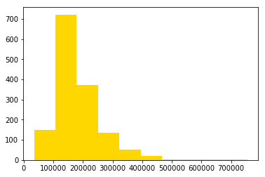
The distribution is positively skewed (a longer tail on the right), so we need to log-transform the target variable to improve the linearity of the data.
y = np.log(train['SalePrice'].ravel()).copy()
Now back to features.
from sklearn.preprocessing import StandardScaler
from sklearn.linear_model import LinearRegression, Lasso
from sklearn.model_selection import cross_val_score, cross_val_predict
from sklearn.decomposition import PCA
from sklearn.feature_selection import RFE
# CONVENTIONAL
quality = train[['OverallQual', 'KitchenQual', 'ExterQual', 'LowQualFinSF', 'HeatingQC']]
footage = train[['TotalBsmtSF', 'GrLivArea', 'GarageArea', 'PoolArea', 'LotArea']]
neighborhood = train[['MSSubClass', 'LandContour', 'Neighborhood', 'BldgType']]
age = train[['YearBuilt', 'YearRemodAdd', 'YrSold']]
property_attr = train[['Foundation', 'Exterior1st', 'Utilities']]
rooms = train[['FullBath', 'BedroomAbvGr', 'Fireplaces', 'GarageCars']]
conventional = pd.get_dummies(pd.concat([quality, footage, neighborhood, age, property_attr, rooms], axis=1))

# ALL
allfeatures = pd.get_dummies(train[[col for col in train.columns if col !='SalePrice']].copy(), drop_first=True)

# CORRELATED
top24 = ss.fit_transform(pd.get_dummies(train[['OverallQual', 'GrLivArea', 'TotalBsmtSF', 'GarageCars', 'GarageArea',
                    '1stFlrSF', 'FullBath', 'TotRmsAbvGrd', 'YearBuilt', 'YearRemodAdd',
                    'Fireplaces', 'BsmtFinSF1', 'LotFrontage', 'SaleCondition', 'WoodDeckSF',
                    '2ndFlrSF', 'OpenPorchSF', 'HalfBath', 'LotArea', 'BsmtFullBath',
                    'BsmtUnfSF', 'BedroomAbvGr', 'ScreenPorch', 'PoolArea']]))
ss = StandardScaler()
allfeatures_scaled = ss.fit_transform(allfeatures)
conventional_scaled = ss.fit_transform(conventional)
top24_scaled = ss.fit_transform(top24)
# PCA
pca = PCA(n_components=24)
pca_features = pca.fit_transform(allfeatures_scaled)

# RFE
rfe = RFE(lr, n_features_to_select=48)
rfe.fit(allfeatures_scaled, y)
rfe_features = allfeatures.iloc[:, rfe.support_]

# Lasso
from sklearn.feature_selection import SelectFromModel
lasso = Lasso()
lasso.fit(allfeatures, y)
lasso_features = SelectFromModel(lasso, prefit=True).transform(allfeatures_scaled)
print("%s variables of %s were removed"%(sum(lasso.coef_ == 0), len(lasso.coef_)),'\n')

# To see columns chosen by Lasso
for col, coef in zip(allfeatures.columns, lasso.coef_):
        if coef != 0.0:
            print('Use', col, coef)
182 variables of 194 were removed

Use Id -9.25448035226e-06
Use LotArea 1.57170015403e-06
Use YearBuilt 0.00251265135532
Use YearRemodAdd 0.00124464719792
Use BsmtFinSF1 4.75616875206e-05
Use TotalBsmtSF 0.000163445309797
Use 2ndFlrSF 2.24344702183e-05
Use GrLivArea 0.000310610759168
Use GarageArea 0.000386175392281
Use WoodDeckSF 0.000159391904829
Use ScreenPorch 0.00013472881683
Use MiscVal -5.63585179224e-08
SCORING
# Baseline model predicting the mean
from sklearn.metrics import r2_score
train['baseline'] = y.mean()
print('Score of predicting the mean:', r2_score(train['SalePrice'], train['baseline']))
Score of predicting the mean: -5.18642379411
# Just the Linear Regression model
lr = LinearRegression()
print('Score of LR using all features:', cross_val_score(lr, allfeatures_scaled, y, cv=5).mean())
print('Score of LR using conventional features:', cross_val_score(lr, conventional_scaled, y, cv=5).mean())
print('Score LR via .corr:', cross_val_score(lr, top24_scaled, y, cv=5).mean())
Score of LR using all features: -3.42869523964e+25
Score of LR using conventional features: -9.14521643608e+25
Score LR via .corr: 0.830148489466
print('Score via PCA:', cross_val_score(lr, pca_features, y, cv=5).mean())
Score via PCA: 0.822915445903
print('Score via Lasso:', cross_val_score(lr, lasso_features, y, cv=5).mean())
Score via Lasso: 0.768549011367
print('Score via RFE:', cross_val_score(lr, rfe_features, y, cv=5).mean())
Score via RFE: 0.787283940054
Same in a PIPELINE
from sklearn.preprocessing import Imputer
from sklearn.pipeline import Pipeline
X = allfeatures
imputing = ('imputing', Imputer(missing_values=0, strategy='mean', axis=0))
scaling = ('scaling', StandardScaler())
rfe = ('rfe', RFE(lr, n_features_to_select=24, step=5))
pca = ('pca', PCA(n_components=24))
lrp = ('lrp', LinearRegression())
lasso = ('lasso', Lasso())

lr_pipeline = Pipeline([imputing, scaling, lrp])
lr_pipeline.fit(conventional, y)

rfe_pipeline = Pipeline([imputing, scaling, rfe]) # Create the pipeline: pipeline
rfe_pipeline.fit(X, y) # Fit the pipeline to the train set

pca_pipeline = Pipeline([imputing, scaling, pca, lrp])
pca_pipeline.fit(X, y)

lasso_pipeline = Pipeline([imputing, scaling, lasso]) # Create the pipeline: pipeline
lasso_features = SelectFromModel(Lasso().fit(X, y), prefit=True).transform(X)

print('LR score, conv:', cross_val_score(lr_pipeline, conventional, y, cv=5).mean())
print('LR score, top24:', cross_val_score(lr_pipeline, top24, y, cv=5).mean())
print('PCA score:', cross_val_score(pca_pipeline, X, y, cv=5).mean())
print('RFE score:', cross_val_score(rfe_pipeline, X, y).mean())
print('Lasso score:', cross_val_score(lr, lasso_features, y, cv=5).mean())
LR score, conv: 0.812249293965
LR score, top24: 0.830349597185
PCA score: 0.802999116798
RFE score: 0.822382038559
Lasso score: 0.768549011367